Dynamic Hedge Ratios with a Kalman Filter

I built this project to better understand how hedge ratios evolve when the relationship between two markets changes over time.

The notebook constructs equal-weight US and European energy-equity baskets, converts European prices into US dollars, and compares static OLS, rolling OLS and a Kalman filter.

Each model generates a mean-reversion signal evaluated through a causal walk-forward backtest. Signals are executed on the following day, portfolio exposure is normalised, and transaction costs include entries, exits and hedge-ratio rebalancing.

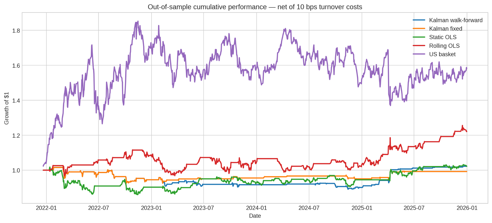
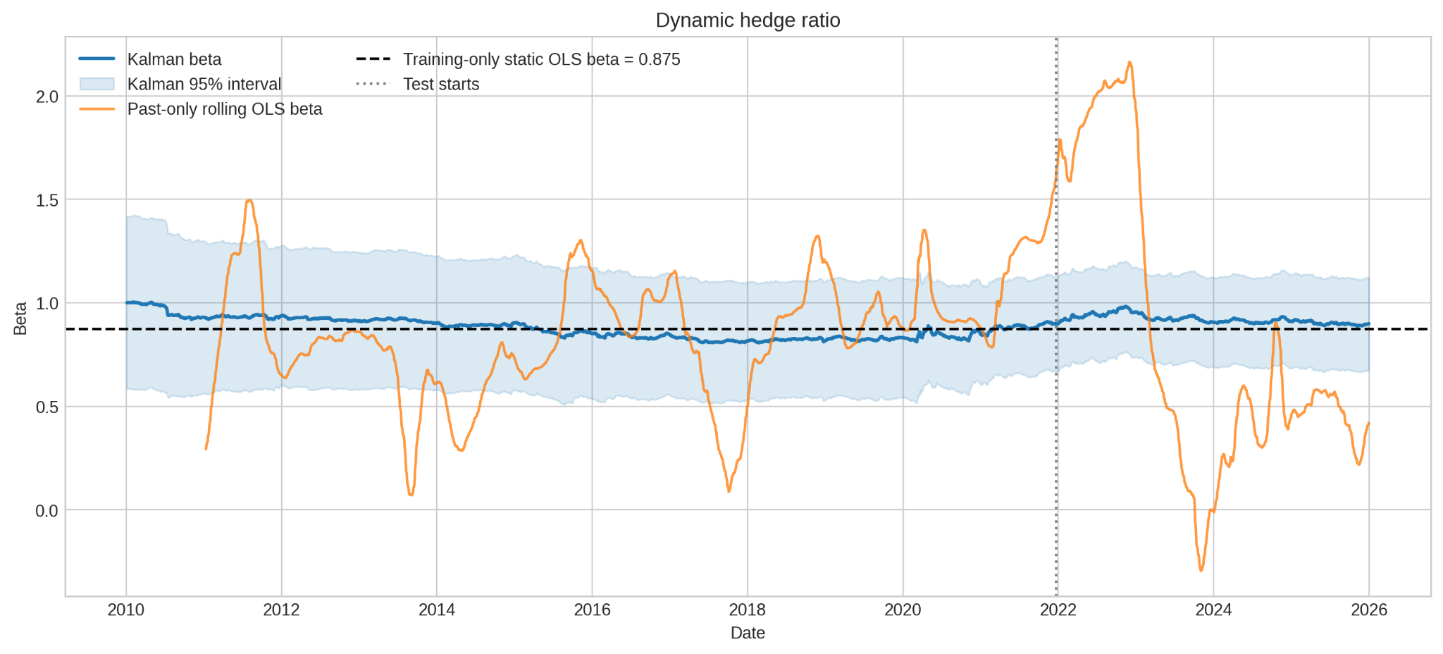
The Kalman filter produces a more stable hedge ratio than rolling OLS. In this dataset, however, rolling OLS delivers the strongest out-of-sample performance. Bootstrap intervals and cost-sensitivity tests leave substantial statistical uncertainty.

What I wanted to understand

Compare how a state-space model and two OLS baselines estimate a changing hedge ratio, then test whether smoother estimates translate into better out-of-sample results.

What the project covers

1. Build equal-weight US and European energy-equity baskets and convert European prices into US dollars.
2. Estimate static OLS, past-only rolling OLS and Kalman state-space hedge ratios.
3. Generate mean-reversion signals from standardised one-step-ahead innovations and select parameters causally through walk-forward validation.
4. Execute signals on the next day, normalise portfolio exposure and charge transaction costs for entries, exits and hedge-ratio rebalancing.
5. Run Engle–Granger and ADF diagnostics, moving-block bootstrap intervals, and cost and parameter sensitivity tests.

What came out of the comparison

• Kalman walk-forward Sharpe: approximately 0.12.
• Fixed Kalman Sharpe: approximately 0.00.
• Rolling OLS Sharpe: approximately 0.51, with cumulative performance of approximately +23% in the test sample.
• Every moving-block bootstrap confidence interval includes zero.
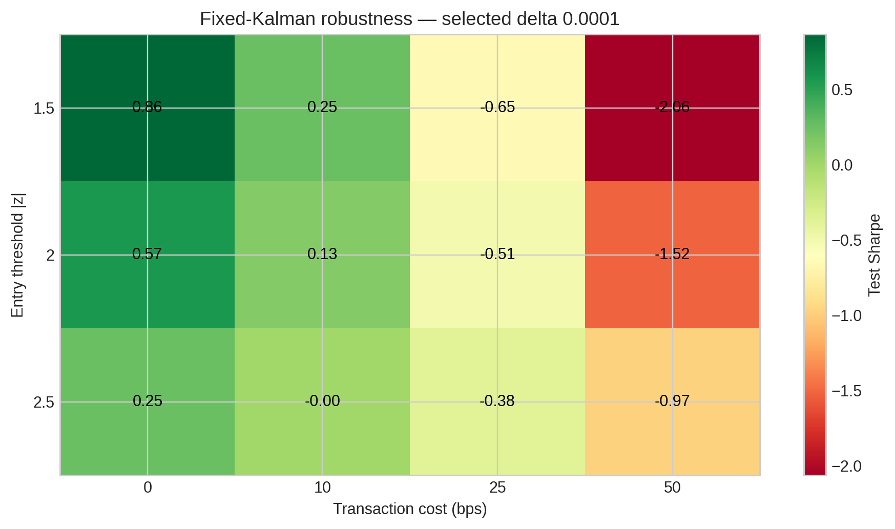
• Kalman results deteriorate materially as assumed transaction costs increase.

The useful conclusion is methodological: Kalman filtering stabilises the estimated hedge ratio, but greater model stability does not automatically produce better trading performance. These are comparative out-of-sample results, not evidence of a reliably profitable strategy.

innovation = y_t - (alpha_pred + beta_pred * x_t)
z_score = innovation / np.sqrt(innovation_variance)

position = signal.shift(1).fillna(0.0)
net_return = gross_return - turnover * cost_bps * 1e-4

What the result does not claim

The exercise uses equal-weight baskets, simplified execution assumptions and one historical sample. Model rankings are sensitive to thresholds and transaction costs, while the bootstrap intervals show that the observed Sharpe ratios are not statistically precise.